These datasets contain grid cells covering the EU and neighbouring countries at resolutions from 1 km to 100 km. Population figures are available for selected reference years.
Arguments
- resolution
The grid cell resolution in km. Available values are
"1","2","5","10","20","50"and"100". See Details.- spatialtype
A character string selecting
"REGION"or"POINT".- cache_dir
A character string with a path to a cache directory. See Caching strategies section in
gisco_set_cache_dir().- update_cache
A logical value indicating whether to refresh the cached file. Defaults to
FALSE. When set toTRUE, it forces a new download.- verbose
A logical value indicating whether to display informational messages.
Value
A sf object.
Details
gisco_get_grid() downloads the GeoPackage representation of the grid as
polygon cells (spatialtype = "REGION") or cell-centre points
(spatialtype = "POINT"). The official distribution also provides tabular
CSV and Parquet files, which this function does not download.
All grid geometries use EPSG:3035. Population
columns are named TOT_P_YYYY, where YYYY is the reference year. To
calculate population density, divide a population value by the cell area in
square kilometres (resolution^2).
The file sizes range from 428 KB (resolution = 100)
to 1.7 GB (resolution = 1).
Copyright
Population variables (TOT_P_*) have year- and country-specific licensing
conditions. Other grid elements are covered by the general Eurostat
copyright provisions. Review the licensing table and metadata on the
official grid page before redistributing or publishing the data.
Examples
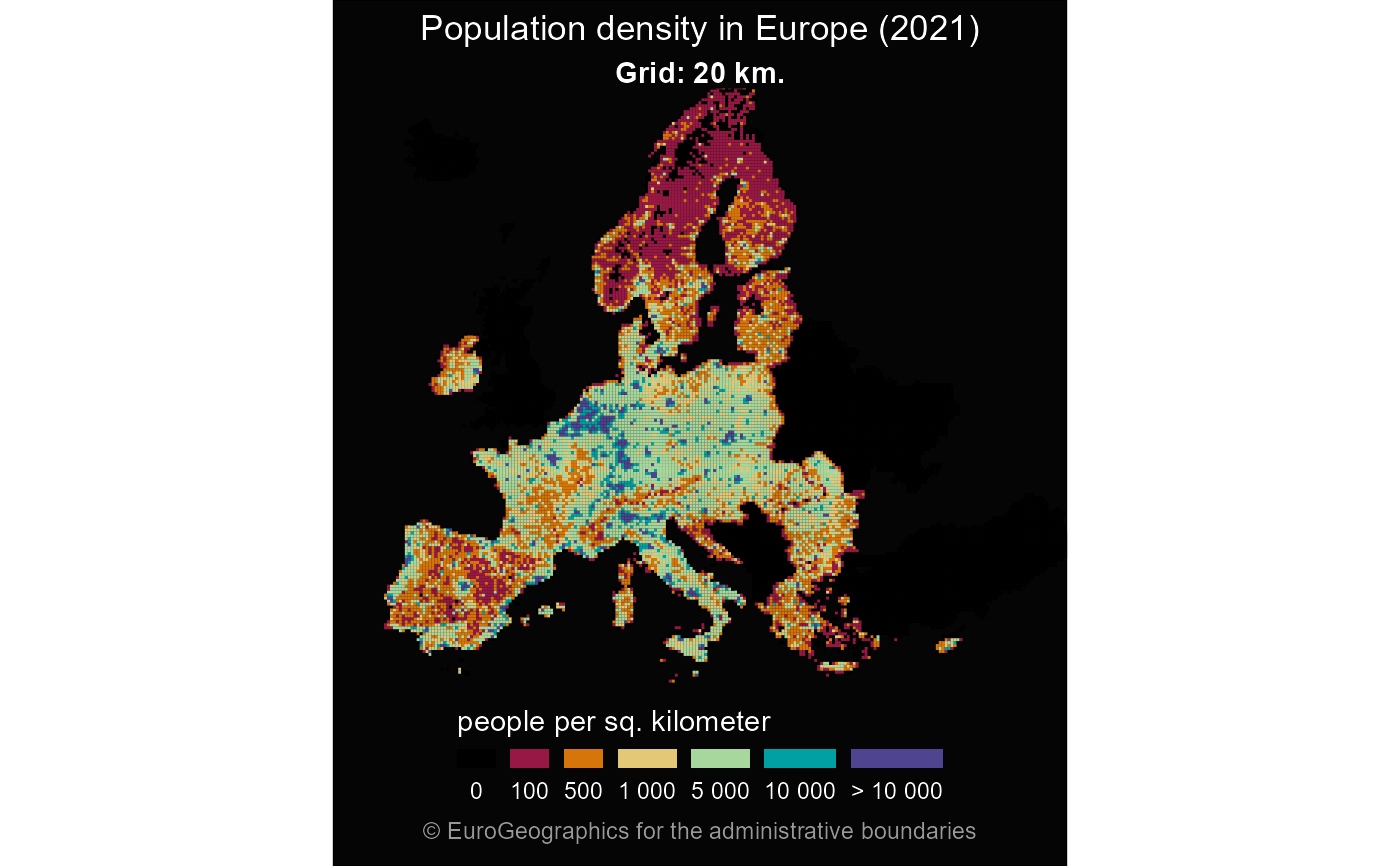
grid <- gisco_get_grid(resolution = 20)

# Proceed if downloaded correctly.
if (
  !is.null(grid) &&
    requireNamespace("dplyr", quietly = TRUE) &&
    requireNamespace("ggplot2", quietly = TRUE)
) {
  library(dplyr)

  grid <- grid |>
    mutate(popdens = TOT_P_2021 / 20^2)

  breaks <- c(0, 1, 10, 25, 50, 100, 250, 500, 1000, Inf)

  # Cut groups.
  grid <- grid |>
    mutate(popdens_cut = cut(popdens,
      breaks = breaks,
      include.lowest = TRUE
    ))

  cut_labs <- prettyNum(breaks, big.mark = " ")[-1]
  cut_labs[1] <- "0"
  cut_labs[9] <- "> 1000"

  pal <- c(
    "black",
    hcl.colors(length(breaks) - 2, palette = "Spectral", alpha = 0.9)
  )

  library(ggplot2)

  ggplot(grid) +
    geom_sf(aes(fill = popdens_cut), color = NA, linewidth = 0) +
    coord_sf(
      xlim = c(2500000, 7000000),
      ylim = c(1500000, 5200000)
    ) +
    scale_fill_manual(
      values = pal, na.value = "black",
      name = "",
      labels = cut_labs
    ) +
    theme_void() +
    labs(
      title = "Population density in Europe (2021)",
      subtitle = "Grid: 20 km. People by square km.",
      caption = paste(
        "Source: Eurostat GISCO grid dataset.\n",
        "Review the applicable population-data licence."
      )
    ) +
    theme(
      text = element_text(colour = "white"),
      plot.background = element_rect(fill = "grey2"),
      plot.title = element_text(hjust = 0.5),
      plot.subtitle = element_text(hjust = 0.5, face = "bold"),
      plot.caption = element_text(
        color = "grey60", hjust = 0.5, vjust = 0,
        margin = margin(t = 5, b = 10)
      ),
      legend.key.height = unit(0.5, "lines"),
      legend.key.width = unit(1, "lines")
    )
}