Get grid cells covering covering Europe for various resolutions

These datasets contain grid cells covering the European land territory, for various resolutions from 1km to 100km. Base statistics such as population figures are provided for these cells.

Usage

gisco_get_grid(
  resolution = "20",
  spatialtype = c("REGION", "POINT"),
  cache_dir = NULL,
  update_cache = FALSE,
  verbose = FALSE
)

Source

https://ec.europa.eu/eurostat/web/gisco/geodata/reference-data/grids

Arguments

resolution: Resolution of the grid cells on kms. Available values are "1", "2", "5", "10", "20", "50", "100". See Details.
spatialtype: Select one of "REGION" or "POINT".
cache_dir: A path to a cache directory. See About caching.
update_cache: A logical whether to update cache. Default is FALSE. When set to TRUE it would force a fresh download of the source .geojson file.
verbose: Logical, displays information. Useful for debugging, default is FALSE.

Value

A POLYGON/POINT

sf object.

Details

Files are distributed on EPSG:3035.

The file sizes range is from 428Kb (resolution = "100") to 1.7Gb resolution = "1". For resolutions 1km and 2km you would need to confirm the download.

Note

There are specific downloading provisions, please see https://ec.europa.eu/eurostat/web/gisco/geodata/reference-data/grids

About caching

You can set your cache_dir with gisco_set_cache_dir().

Sometimes cached files may be corrupt. On that case, try re-downloading the data setting update_cache = TRUE.

If you experience any problem on download, try to download the corresponding .geojson file by any other method and save it on your cache_dir. Use the option verbose = TRUE for debugging the API query.

For a complete list of files available check gisco_db.

Author

dieghernan, https://github.com/dieghernan/

Examples

# \donttest{
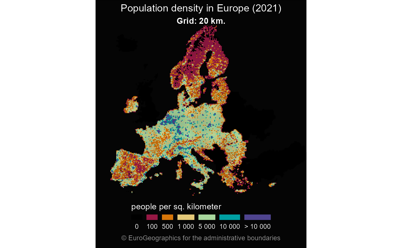
grid <- gisco_get_grid(resolution = 20)
#> Warning: GDAL Message 1: GPKG: unrecognized user_version=0x00000000 (0) on 'C:\Users\runneradmin\AppData\Local\Temp\RtmpMxaj0I\giscoR\pkgdown\grid_20km_surf.gpkg'

# If downloaded correctly proceed

if (!is.null(grid)) {
  library(dplyr)

  grid <- grid %>%
    mutate(popdens = TOT_P_2021 / 20)

  breaks <- c(0, 0.1, 100, 500, 1000, 5000, 10000, Inf)

  # Cut groups
  grid <- grid %>%
    mutate(popdens_cut = cut(popdens,
      breaks = breaks,
      include.lowest = TRUE
    ))

  cut_labs <- prettyNum(breaks, big.mark = " ")[-1]
  cut_labs[1] <- "0"
  cut_labs[7] <- "> 10 000"

  pal <- c("black", hcl.colors(length(breaks) - 2,
    palette = "Spectral",
    alpha = 0.9
  ))

  library(ggplot2)

  ggplot(grid) +
    geom_sf(aes(fill = popdens_cut), color = NA, linewidth = 0) +
    coord_sf(
      xlim = c(2500000, 7000000),
      ylim = c(1500000, 5200000)
    ) +
    scale_fill_manual(
      values = pal, na.value = "black",
      name = "people per sq. kilometer",
      labels = cut_labs,
      guide = guide_legend(
        direction = "horizontal",
        nrow = 1
      )
    ) +
    theme_void() +
    labs(
      title = "Population density in Europe (2021)",
      subtitle = "Grid: 20 km.",
      caption = gisco_attributions()
    ) +
    theme(
      text = element_text(colour = "white"),
      plot.background = element_rect(fill = "grey2"),
      plot.title = element_text(hjust = 0.5),
      plot.subtitle = element_text(hjust = 0.5, face = "bold"),
      plot.caption = element_text(
        color = "grey60", hjust = 0.5, vjust = 0,
        margin = margin(t = 5, b = 10)
      ),
      legend.position = "bottom",
      legend.title.position = "top",
      legend.text.position = "bottom",
      legend.key.height = unit(0.5, "lines"),
      legend.key.width = unit(1, "lines")
    )
}
#> 
#> Attaching package: 'dplyr'
#> The following objects are masked from 'package:stats':
#> 
#>     filter, lag
#> The following objects are masked from 'package:base':
#> 
#>     intersect, setdiff, setequal, union

# }