Introduction
The full site with more examples and vignettes is available at https://ropengov.github.io/giscoR/.
giscoR is a package designed to provide a simple interface to the Eurostat GISCO geodata distribution.
GISCO provides geospatial data for the European Union, its member states and subnational regions. It supplies geospatial files in different formats, with a focus on Europe and global datasets such as country boundaries, labels and coastal lines.
GISCO supplies data at multiple resolutions: high-resolution datasets for small areas (01M, 03M) and lighter datasets for larger areas (10M, 20M, 60M). Datasets are available in three coordinate reference systems: EPSG:4326, EPSG:3035 and EPSG:3857.
giscoR returns sf package objects. See https://r-spatial.github.io/sf/ for details.
Caching
giscoR supports caching downloaded datasets. Set the cache directory with:
gisco_set_cache_dir("./path/to/location")If a file is not available locally, it is downloaded to that directory so subsequent requests for the same data can read from the local cache.
If downloading fails, you can manually download the file from the GISCO geodata distribution and place it in your local cache directory.
Downloading data
Review the following attribution and licensing requirements before using GISCO data:
General copyright
Eurostat’s general copyright notice and license policy applies. Some datasets have additional download and usage provisions. The download and use of these data are subject to acceptance of those provisions. See the administrative units and statistical units for more details.
The gisco_attributions() function provides guidance on this topic and returns attribution text in several languages.
library(giscoR)
c(
  gisco_attributions(lang = "en"),
  gisco_attributions(lang = "fr"),
  gisco_attributions(lang = "de")
) |> cat(sep = "\n\n")
#> © EuroGeographics for the administrative boundaries
#>
#> © EuroGeographics pour les limites administratives
#>
#> © EuroGeographics bezüglich der Verwaltungsgrenzen
Basic example
The following example downloads EU member states and candidate countries for 2024.
library(dplyr)
library(ggplot2)
world <- gisco_get_countries(resolution = 3, epsg = 3035)

world <- world |>
  mutate(
    status = case_when(
      EU_STAT == "T" ~ "Current members",
      CC_STAT == "T" ~ "Candidate countries",
      TRUE ~ NA
    ),
    # Set levels.
    status = factor(status,
      levels = c("Current members", "Candidate countries")
    )
  )

ggplot(world) +
  geom_sf(fill = "#c1c1c1") +
  geom_sf(aes(fill = status), color = "white") +
  guides(fill = guide_legend(direction = "horizontal")) +
  # Center on Europe with EPSG 3035.
  coord_sf(
    xlim = c(2377294, 7453440),
    ylim = c(1313597, 5628510)
  ) +
  scale_fill_manual(
    values = c("#039", "#2782bb"), na.value = "#c1c1c1",
    na.translate = FALSE
  ) +
  theme_minimal() +
  theme(
    panel.background = element_rect(fill = "grey90", color = NA),
    axis.line = element_blank(),
    axis.text = element_blank(),
    panel.grid = element_blank(),
    legend.position = "bottom"
  ) +
  labs(
    title = "EU member states and candidate countries (2024)",
    caption = gisco_attributions(),
    fill = ""
  )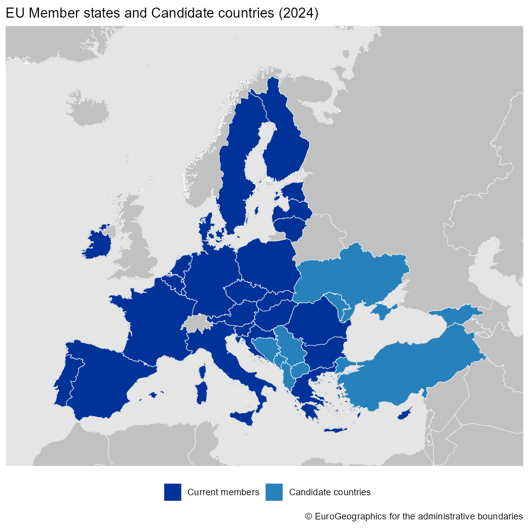
EU member states and candidate countries (2024)
You can select specific countries by name in any language, ISO 3166-1 alpha-3 codes or Eurostat codes. However, you cannot mix these identifier types in a single call.
You can also combine datasets by using the same resolution, epsg and (optionally) year:
cntr <- c("Morocco", "Algeria", "Tunisia", "Libya", "Egypt")

africa_north <- gisco_get_countries(
  country = cntr,
  resolution = "03",
  epsg = "4326", year = "2024"
)

# Order plot facets.
africa_north$NAME_ENGL <- factor(africa_north$NAME_ENGL, levels = cntr)

# Get coastal lines.
coast <- gisco_get_coastal_lines(
  resolution = "03",
  epsg = "4326",
  year = "2016"
)

# Create plot.
ggplot(coast) +
  geom_sf(color = "#B9B9B9") +
  geom_sf(data = africa_north, fill = "#346733", color = "#335033") +
  coord_sf(xlim = c(-13, 37), ylim = c(18.5, 40)) +
  facet_wrap(vars(NAME_ENGL), ncol = 2) +
  labs(caption = gisco_attributions("fr"))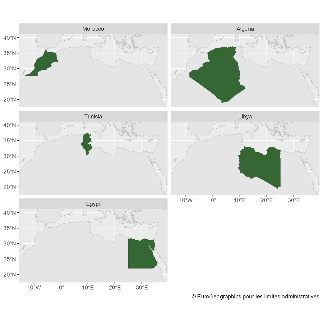
Political map of North Africa
Thematic maps with giscoR
This example shows how giscoR can be used with Eurostat data. For plotting, we use the ggplot2 package. Any package that supports sf package objects, such as tmap, mapsf or leaflet, can be used.
# Load EU member data.
library(giscoR)
library(dplyr)
library(eurostat)
library(ggplot2)

nuts2 <- gisco_get_nuts(
  year = "2021", epsg = "3035", resolution = "10",
  nuts_level = "2"
)
# Get country borders.
borders <- gisco_get_countries(epsg = "3035", year = "2020", resolution = "3")

eu_bord <- borders |>
  filter(CNTR_ID %in% nuts2$CNTR_CODE)

# Retrieve disposable income data from Eurostat.
pps <- get_eurostat("tgs00026") |>
  filter(TIME_PERIOD == "2022-01-01")
#>
indexed 0B in  0s, 0B/s
indexed 2.15GB in  0s, 2.15GB/s


nuts2_sf <- nuts2 |>
  left_join(pps, by = "geo") |>
  mutate(
    values_th = values / 1000,
    categ = cut(values_th, c(0, 15, 30, 60, 90, 120, Inf))
  )

# Adjust labels.
labs <- levels(nuts2_sf$categ)
labs[1] <- "< 15"
labs[6] <- "> 120"
levels(nuts2_sf$categ) <- labs

# Create the plot.
ggplot(nuts2_sf) +
  # Add background geometry.
  geom_sf(data = borders, fill = "#e1e1e1", color = NA) +
  geom_sf(aes(fill = categ), color = "grey20", linewidth = .1) +
  geom_sf(data = eu_bord, fill = NA, color = "black", linewidth = .15) +
  # Center on Europe with EPSG 3035.
  coord_sf(xlim = c(2377294, 6500000), ylim = c(1413597, 5228510)) +
  # Configure legends and color.
  scale_fill_manual(
    values = hcl.colors(length(labs), "Geyser", rev = TRUE),
    # Label missing values.
    labels = function(x) {
      ifelse(is.na(x), "No Data", x)
    },
    na.value = "#e1e1e1"
  ) +
  guides(fill = guide_legend(nrow = 1)) +
  theme_void() +
  theme(
    text = element_text(colour = "grey0"),
    panel.background = element_rect(fill = "#97dbf2"),
    panel.border = element_rect(fill = NA, color = "grey10"),
    plot.title = element_text(hjust = 0.5, vjust = -1, size = 12),
    plot.subtitle = element_text(
      hjust = 0.5, vjust = -2, face = "bold",
      margin = margin(b = 10, t = 5), size = 12
    ),
    plot.caption = element_text(
      size = 8, hjust = 0, margin =
        margin(b = 4, t = 8)
    ),
    legend.text = element_text(size = 7, ),
    legend.title = element_text(size = 7),
    legend.position = "bottom",
    legend.direction = "horizontal",
    legend.text.position = "bottom",
    legend.title.position = "top",
    legend.key.height = rel(0.5),
    legend.key.width = unit(0.1, "npc")
  ) +
  # Add labels.
  labs(
    title = "Disposable income of private households (2022)",
    subtitle = "NUTS 2 level",
    fill = "euros (thousands)",
    caption = paste0(
      "Source: Eurostat, ", gisco_attributions()
    )
  )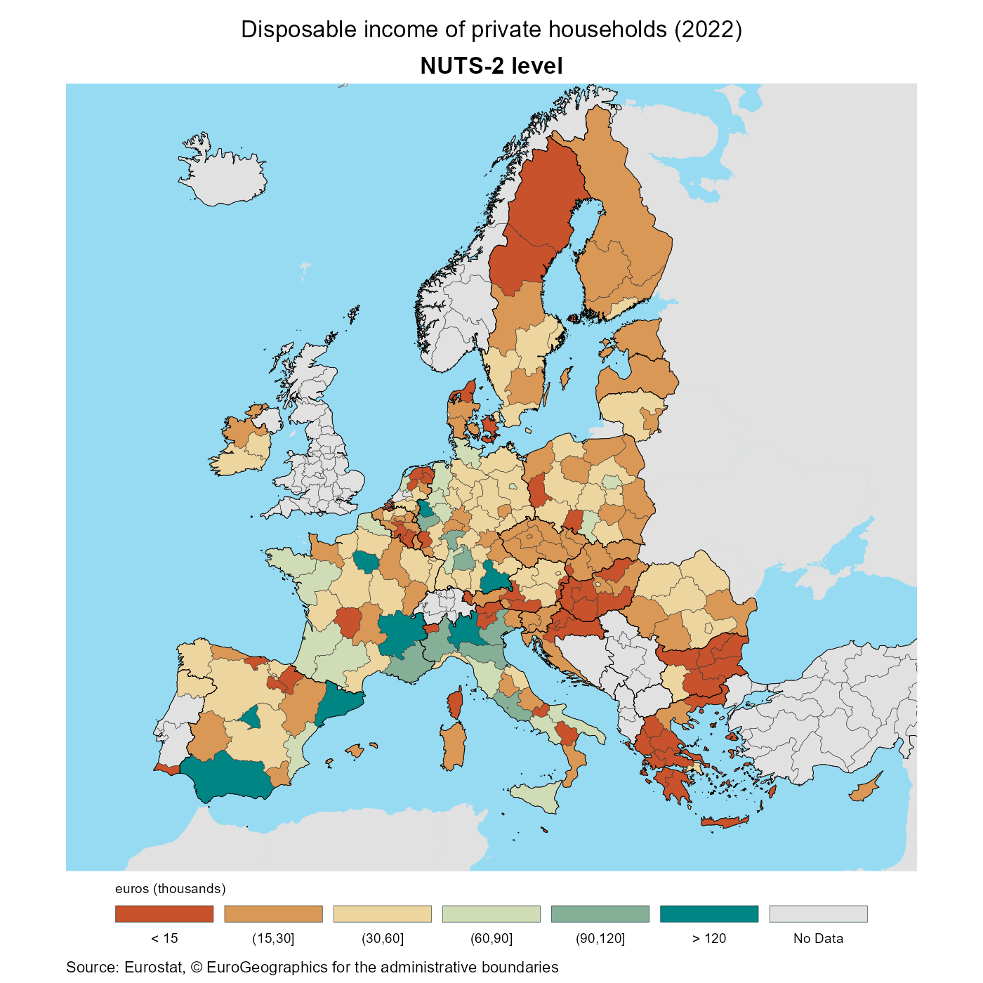
Disposable income of private households by NUTS 2 regions (2022)