fmi2: introduction

Setup

fmi2 is not yet in CRAN, so you’ll need to install it directly from GitHub. While you’re at it, make sure you also install all the packages below as we’ll be using them in this tutorial.

install.packages(c("DT", "ggplot2", "leaflet", "remotes", "sf", "tidyverse"))

remotes::install_github("ropengov/fmi2")
remotes::install_github("ropensci/skimr")

library(DT)
library(fmi2)
library(ggplot2)
library(knitr)
library(leaflet)
library(sf)
library(skimr)

Getting started

You can retrieve weather stating observation data with various temporal resolution using fmi2. First thing you need to know is of course which location exactly you want to get the data from. The FMI API provides multiple different ways of defining the spatial query area:

Bounding box given by coordindates and defining an area
Place name for which to provide data.
FMISID numeric FMI observation station identifier
GEOID numeric geoid of the location
WMO code of the location

We’ll start off by using the FMISID identifies which is given to each FMI observation stations. The online table is also available in fmi2 using the function fmi_stations():

station_data <- fmi2::fmi_stations() 

station_data %>% 
  DT::datatable()

We’re going to pick “Hanko Tulliniemi” as an example here and use its FMISID (100946) to retrieve the data. As you can see from the table above, it also provides the latlon (geographical) coordinates for the observation station. Before we get the actual data, let’s visualize Hanko region.

# Get data for Tulliniemi only
tulliniemi_station <- station_data %>% 
  dplyr::filter(fmisid == 100946)

# Plot on a map using leaflet
leaflet::leaflet(station_data) %>% 
  leaflet::setView(lng = tulliniemi_station$lon, 
                   lat = tulliniemi_station$lat, 
                   zoom = 11) %>% 
  leaflet::addTiles() %>%  
  leaflet::addMarkers(~lon, ~lat, popup = ~name, label = ~as.character(fmisid))

Getting daily weather observation data

Now that we know how the address a specific observation station, we can proceed to getting the actual data. fmi2 providers several functions to retrieving data with different variables and temporal resolution. We’ll start with obs_weather_daily() which returns daily average observation data from a given location. Let’s get the daily weather observation data for the first 6 monhts of 2019:

# Use Hanko Tulliniemi weather station FMISID
tulliniemi_data <- obs_weather_daily(starttime = "2019-01-01",
                                     endtime = "2019-06-30",
                                     fmisid = 100946)

In total, the function returned 1086 observations. You can also note the following:

class(tulliniemi_data)
#> [1] "sf"         "data.frame"

which means that the data returned by obs_weather_daily() is a spatial sf object with the geometry column storing the geographical information of the weather station. We’ll come back to this later. Now we are interested in what kind of data did we actually get? Let’s find out:

unique(tulliniemi_data$variable)
#> [1] "rrday"        "tday"         "snow"         "tmin"         "tmax"        
#> [6] "TG_PT12H_min"

So there are six variables with their corresponding values. fmi2 provides a helper function describe_variables() that can be useful in finding out more about the variables:

var_descriptions <- fmi2::describe_variables(tulliniemi_data$variable)
var_descriptions %>% 
  DT::datatable()

obs_weather_daily() returns data in so called long (or melted) format meaning that all variable (i.e. parameter) names are contained in column variable and corresponding values in value column. You can transform the data into a wide format using tidyr:

wide_data <- tulliniemi_data %>% 
  tidyr::spread(variable, value) %>% 
  # Let's convert the sf object into a regular tibble
  sf::st_set_geometry(NULL)

wide_data %>% 
  DT::datatable()

Looks like there aren’t too much data for rrday, snow or TG_PT12H_min. Let’s have a closer look at the data:

(skimr::skim(wide_data))

Data summary
Name	wide_data
Number of rows	181
Number of columns	7
_______________________
Column type frequency:
Date	1
numeric	6
________________________
Group variables	None

Variable type: Date

skim_variable	n_missing	complete_rate	min	max	median	n_unique
time	0	1	2019-01-01	2019-06-30	2019-04-01	181

Variable type: numeric

skim_variable	n_missing	complete_rate	mean	sd	p0	p25	p50	p75	p100	hist
rrday	181	0	NaN	NA	NA	NA	NA	NA	NA
snow	181	0	NaN	NA	NA	NA	NA	NA	NA
tday	0	1	4.74	6.46	-9.0	0.6	2.8	9.7	17.9	▂▇▇▃▅
TG_PT12H_min	181	0	NaN	NA	NA	NA	NA	NA	NA
tmax	0	1	7.14	6.74	-4.4	2.2	4.5	12.5	20.8	▃▇▃▃▃
tmin	0	1	2.65	6.66	-12.3	-1.8	1.6	7.6	15.9	▂▅▇▃▃

Seems like the above mentioned variables indeed don’t have data between the defined days. Let’s get the same data from a couple of other observation stations around finland. Note that this time we’re using place name instead of a FMISID.

oulu_data <- obs_weather_daily(starttime = "2019-01-01",
                               endtime = "2019-06-30",
                               place = "Oulu")
nuorgam_data <- obs_weather_daily(starttime = "2019-01-01",
                                  endtime = "2019-06-30",
                                  place = "Nuorgam")
# Add location name to each data set and combine them
oulu_data$location <- "Oulu"
nuorgam_data$location <- "Nuorgam"
tulliniemi_data$location <- "Hanko"

all_data <- rbind(tulliniemi_data, oulu_data, nuorgam_data)
# Factorize location and make order explicit
all_data <- all_data %>% 
  dplyr::mutate(location = factor(location, 
                                  levels = c("Nuorgam", "Oulu", "Hanko"),
                                  ordered = TRUE))

Let’s plot the daily temperature data in different locations:

all_data %>% 
  dplyr::filter(variable == "tday" | variable == "tmax" | variable == "tmin") %>% 
  ggplot(aes(x = time, y = value, color = variable)) + 
  geom_line() + facet_wrap(~ location, ncol=1) + ylab("Temperature (C)\n") +
  xlab("\nDate") + theme_minimal()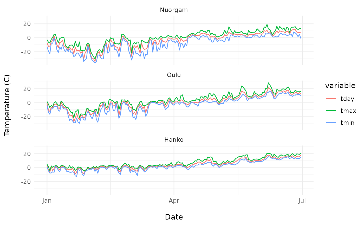

Getting hourly weather observation data

Instead of daily values, it is also possible to retrieve weather observation data with finer temporal resolution, such as hourly data, using the function obs_weather_hourly(). The data retrieved this has slightly different content as compared to the daily data:

# Get the hourly observations for the first day of 2019 in Hanko Tulliniemi
tulliniemi_data <- fmi2::obs_weather_hourly(starttime = "2019-02-01",
                                            endtime = "2019-02-02",
                                            fmisid = 100946)

Again, let’s first have a look at what we actually got:

var_descriptions <- fmi2::describe_variables(tulliniemi_data$variable)
var_descriptions %>% 
  DT::datatable()

Joona Lehtomäki

2023-07-13

Setup

Getting started

Getting daily weather observation data

Getting hourly weather observation data