Spatial data manipulation and analysis R and geofi-package

Installation

geofi can be installed from CRAN using

# install from CRAN
install.packages("geofi")

# Install development version from GitHub
remotes::install_github("ropengov/geofi")

Manuel Gimonds Intro to GIS and Spatial Analysis and especially it’s appendixes provide a good introduction to working with spatial data in R.

Coordinate reference systems

From the book above, have a look at chapter Coordinate Systems in R first.

When using spatial data in R it necessary to have all data in same coordinate reference system (CRS). You can check the CRS of you sf-object with sf::st_crs()-function. All the data you can obtain using geofi is transformed automatically into EPSG:3067. Most of spatial data providers in Finland provide their data in the same CRS.

library(geofi)
library(sf)
library(dplyr)
muni <- get_municipalities()
point <- municipality_central_localities
crs <- st_crs(muni)
crs$input
#> [1] "EPSG:3067"

However, sometimes data is not correctly projected and you have to reproject it using st_transform. Web maps like Google maps or Leaflet use WGS 1984 geographic (long/lat) coordinate system which is fine with added interactive feature, but should be avoided when plotting data on maps elsewhere. This is especially the case with large northern countries like Finland. To demonstrate the effect lets reproject the municipality data to WGS 1984 (usin EPSG code equivalent 4326) and plot it side to side with EPSG:3067

muni_4326 <- st_transform(muni, "EPSG:4326")
crs <- st_crs(muni_4326)
crs$input
#> [1] "EPSG:4326"

library(ggplot2)
  
p1 <- ggplot(muni %>% st_union()) + 
  geom_sf() + 
  labs(subtitle = "EPSG:3067")
p2 <- ggplot(muni_4326 %>% st_union()) + 
  geom_sf() +
  labs(subtitle = "EPSG:4326")
library(patchwork)
wrap_plots(list(p1,p2), nrow = 1) +
  plot_annotation(title = "Map of Finland in two different CRS")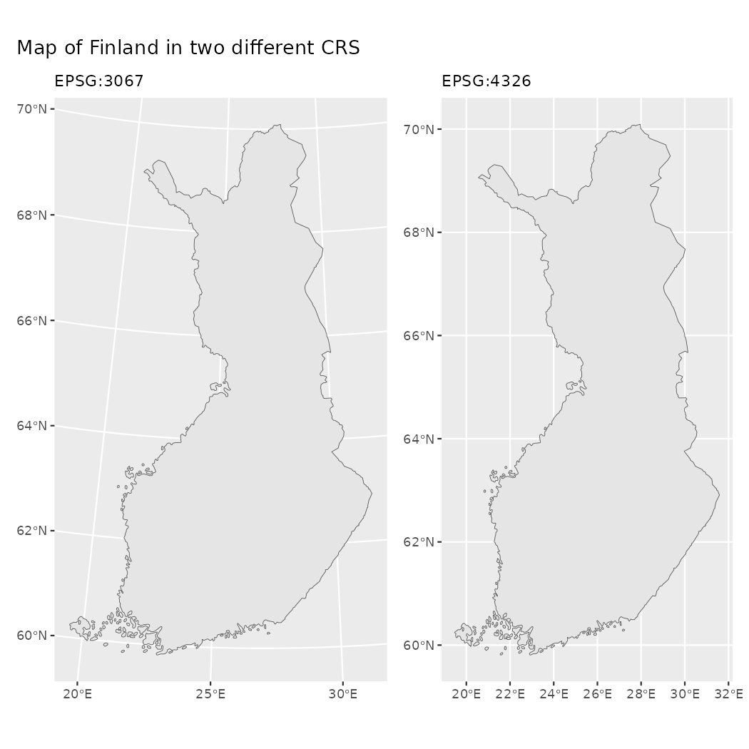

You can see the that northern Finland is larger on the right and the grid below is different.

Area

To compute the area of polygons (municipality in this case), ordering them by size and plotting largest/smalles 10 can be as this.

# compute area
muni$area <- sf::st_area(muni)
# largest
muni %>% 
  arrange(desc(area)) %>% 
  slice(1:10) %>% 
  ggplot() + 
  geom_sf() + 
  geom_sf_label(aes(label = name_fi)) +
  labs(title = "largest 10")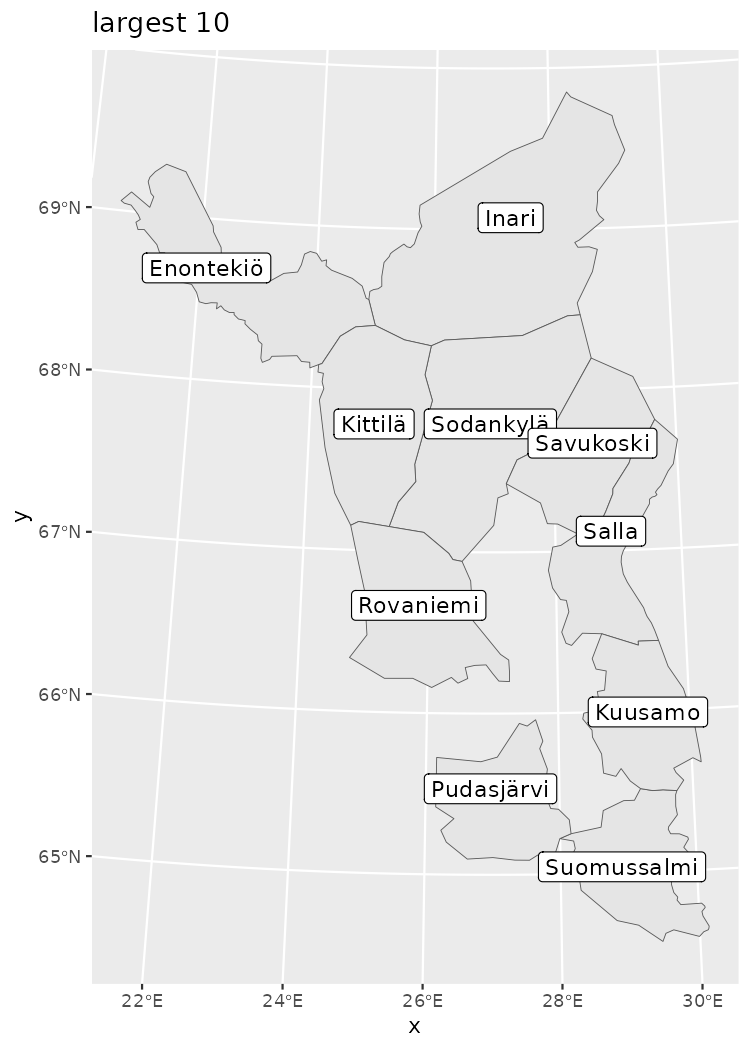

  # smallest
muni %>% 
  arrange(area) %>% 
  slice(1:10) %>% 
  ggplot() + 
  geom_sf() + 
  geom_sf_label(aes(label = name_fi)) +
  labs(title = "smallest 10")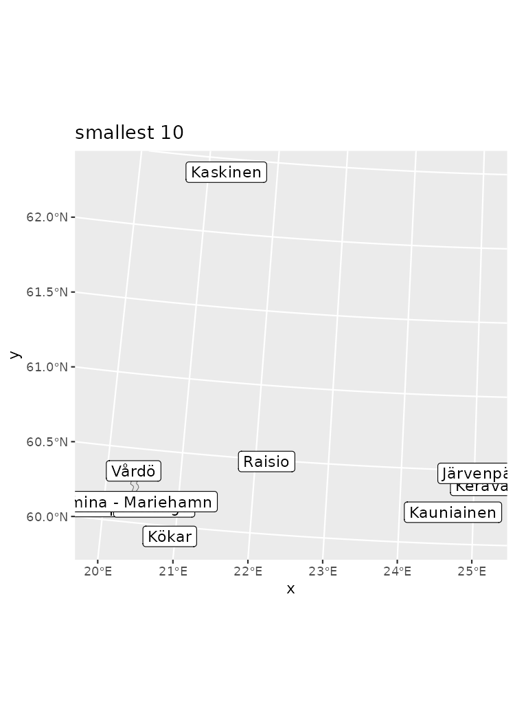

Subsetting

You can subset data your plotting by subsetting your data in conventional filtering codes/names, or you can use geometric operations such as bounding box or intersection.

Lets imagine that we need a more detailed view of the metropolitan area of the Greater Helsinki that consist of the following municipalities: Espoo, Helsinki, Vantaa, Hyvinkää, Järvenpää, Kauniainen, Kerava, Kirkkonummi, Mäntsälä, Nurmijärvi, Pornainen, Sipoo, Tuusula and Vihti. You can subset the data just using the names of municipalities.

greater_helsinki <- c('Espoo','Helsinki','Vantaa','Hyvinkää',
                      'Järvenpää','Kauniainen','Kerava','Kirkkonummi',
                      'Mäntsälä','Nurmijärvi','Pornainen','Sipoo','Tuusula','Vihti')
greater_helsinki_polygon <- muni %>% filter(municipality_name_fi %in% greater_helsinki)

ggplot(greater_helsinki_polygon) + 
  geom_sf() +
  geom_sf(data = point %>% 
            filter(teksti %in% toupper(greater_helsinki)))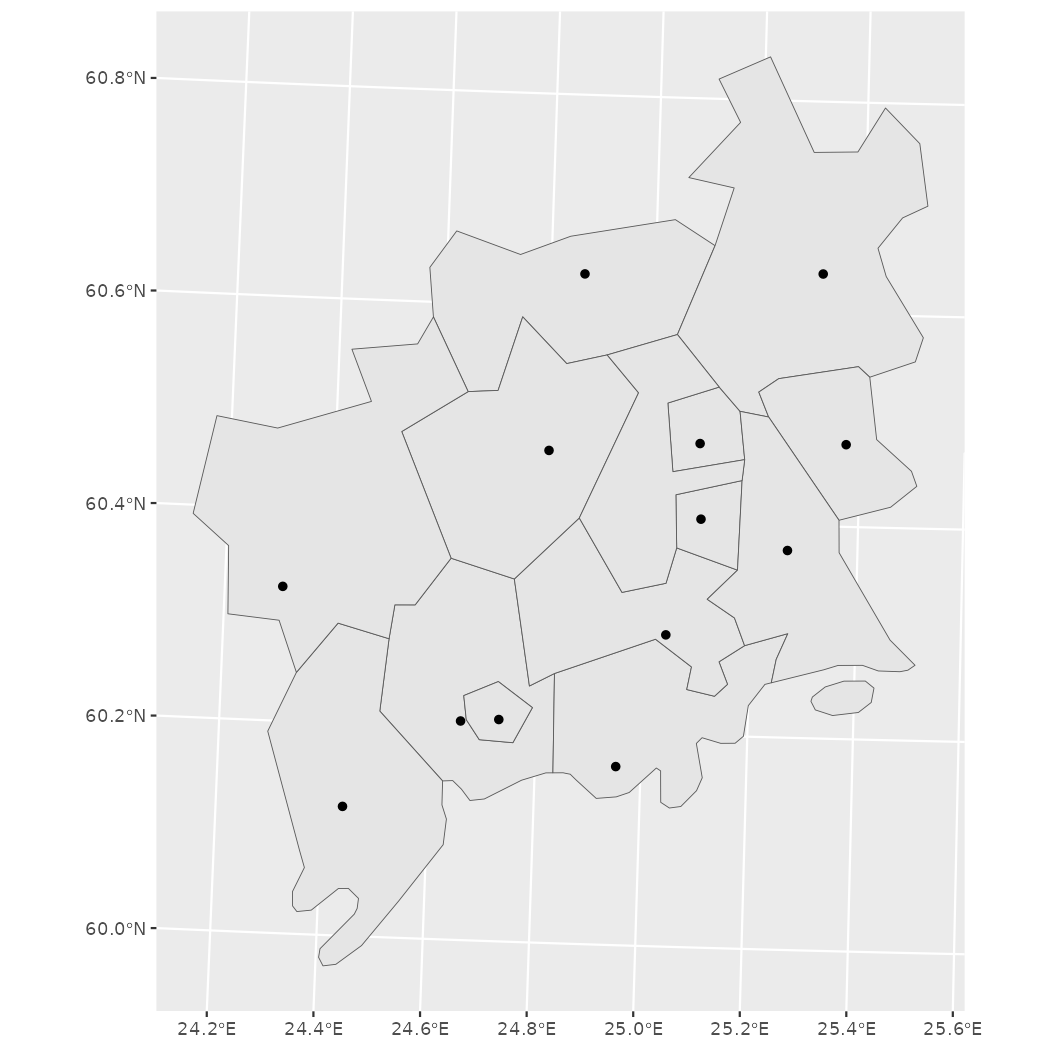

Subsetting using bounding boxes

First, let’s create bounding box from greater Helsinki polygons.

bounding_box_polygon <- st_as_sfc(st_bbox(muni %>% filter(municipality_name_fi %in% greater_helsinki)))

ggplot(st_intersection(bounding_box_polygon, muni)) + 
  geom_sf() +
  geom_sf(data = point %>% filter(teksti %in% toupper(greater_helsinki)))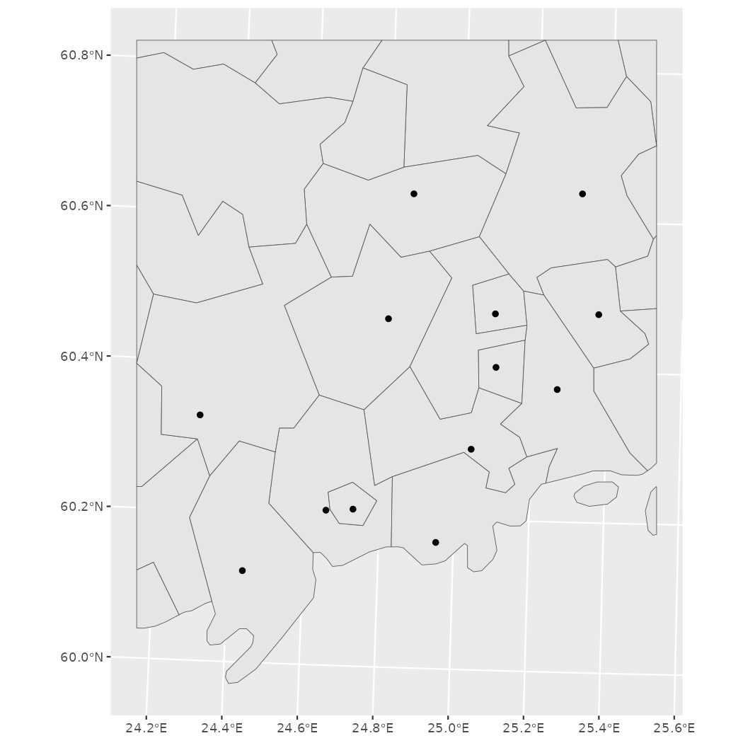

Then, let’s use the point data (municipality central localities) to create the bounding box

bounding_box_point <- st_as_sfc(st_bbox(point %>% filter(teksti %in% toupper(greater_helsinki))))

ggplot(st_intersection(bounding_box_point, muni)) + 
  geom_sf() +
  geom_sf(data = point %>% filter(teksti %in% toupper(greater_helsinki)))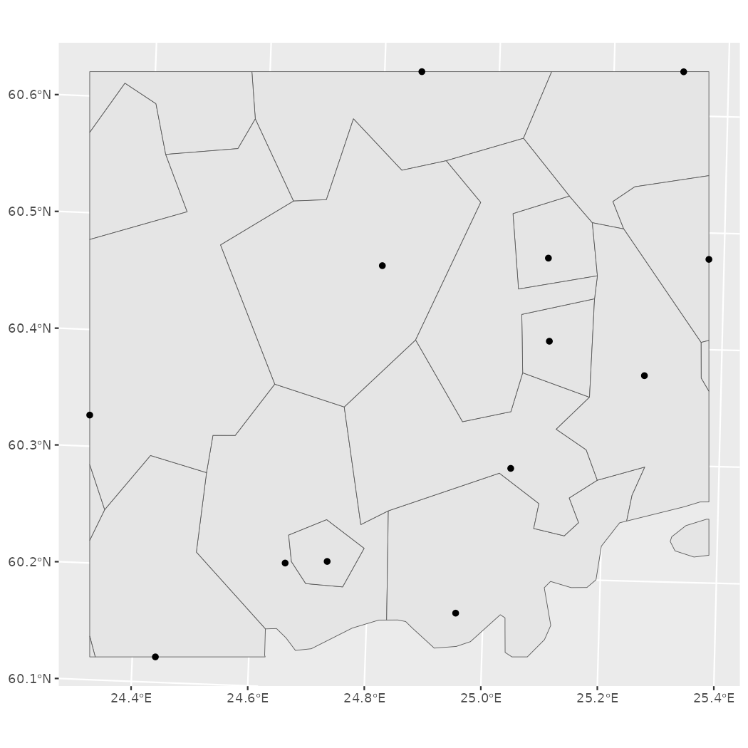

Subsetting neigbours

Neighboring or intersecting objects can be found using st_intersection() in following manner where we plot Helsinki and it’s neighbors.

helsinki <- muni %>%  filter(municipality_name_fi == "Helsinki")
neigbour_codes <- st_intersection(muni,helsinki) %>% 
  pull(municipality_code)

ggplot(muni %>% filter(municipality_code %in% neigbour_codes)) +
  geom_sf() +
  geom_sf_label(aes(label = municipality_name_fi))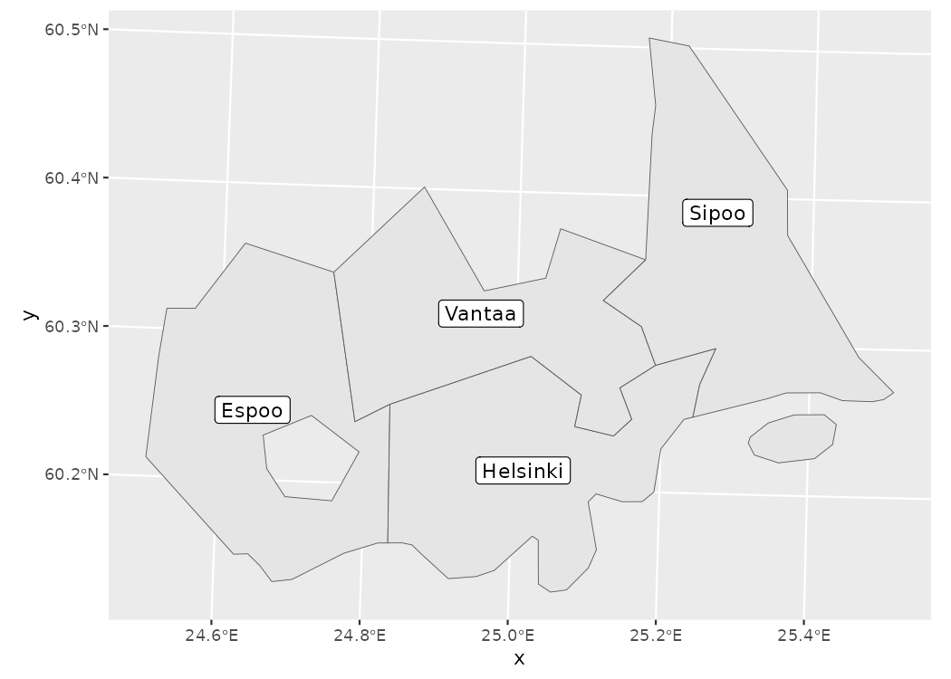

Dissolving polygons (Union)

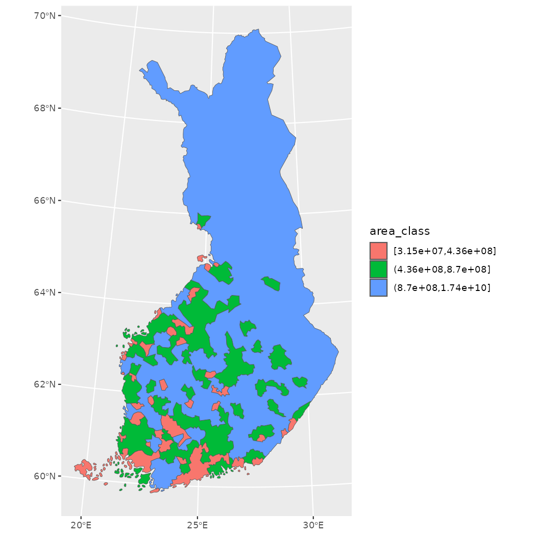
Often there is need to create alternative regional breakdown to existing ones and aggregating data accordingly. First we need to subset the required members and then dissolve them using st_union(). Below we classify municipalities in three equal size categories based on area, dissolve them and plot.

Lets first plot the smallest category as a single multipolygon.

muni$area_class <- cut_number(x = as.numeric(muni$area), n = 3)

muni %>% 
  filter(area_class == levels(muni$area_class)[1]) %>% 
  st_union() %>% 
  ggplot() +
  geom_sf()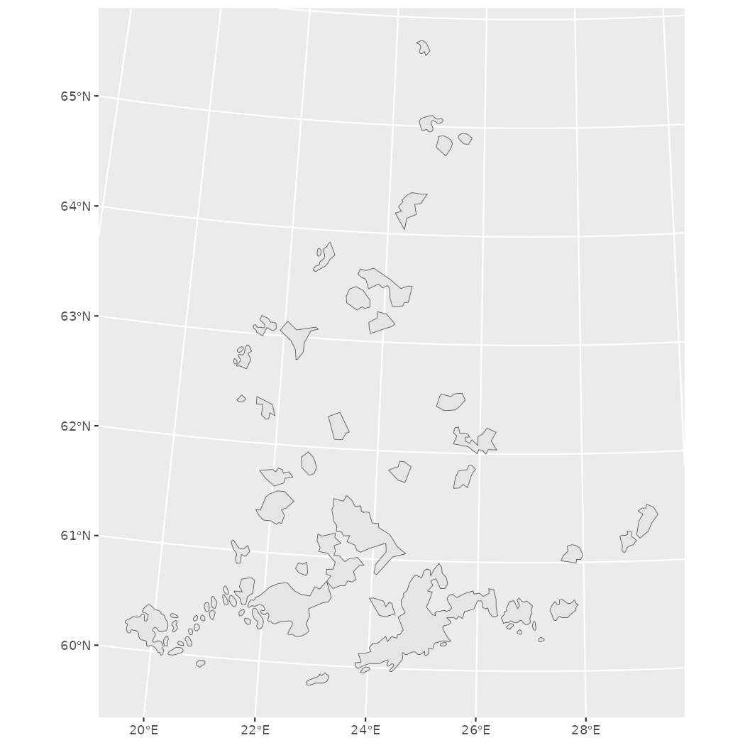

To union all three into same data you can use group_by and summarise

muni %>% 
  group_by(area_class) %>%
  summarise() %>% 
  ggplot() +
  geom_sf(aes(fill = area_class))

Centroids, buffers, grids and voronois

The following operations derive from Marko Kallio’s course at CSC in February 2020 Spatial data analysis with R.

Polygon centroids

geofi contains data on municipality central locations (geofi::municipality_central_localities). Instead of those you may need the actual geographical centers ie. centroids of a polygon that can be computed using st_centroid and plotted with ggplot.

muni_centroids <- st_centroid(muni)

ggplot() +
  geom_sf(data = muni) +
  geom_sf(data = muni_centroids, color = "blue") +
  # plot also the municipality_central_localities
  geom_sf(data = municipality_central_localities, color = "red")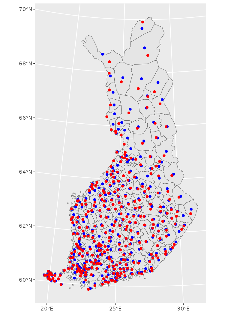

Buffers

Buffers can be useful, for instance, calculating the share of buildings that are within certain radius from central localities. That example is not explained here, but we only show how to create 15km radius around polygon centroids.

muni_centroids_buffer <- muni_centroids %>%
    st_buffer(dist = 15000)

ggplot() +
  geom_sf(data = muni) +
  geom_sf(data = muni_centroids_buffer) +
  geom_sf(data = muni_centroids, shape = 3)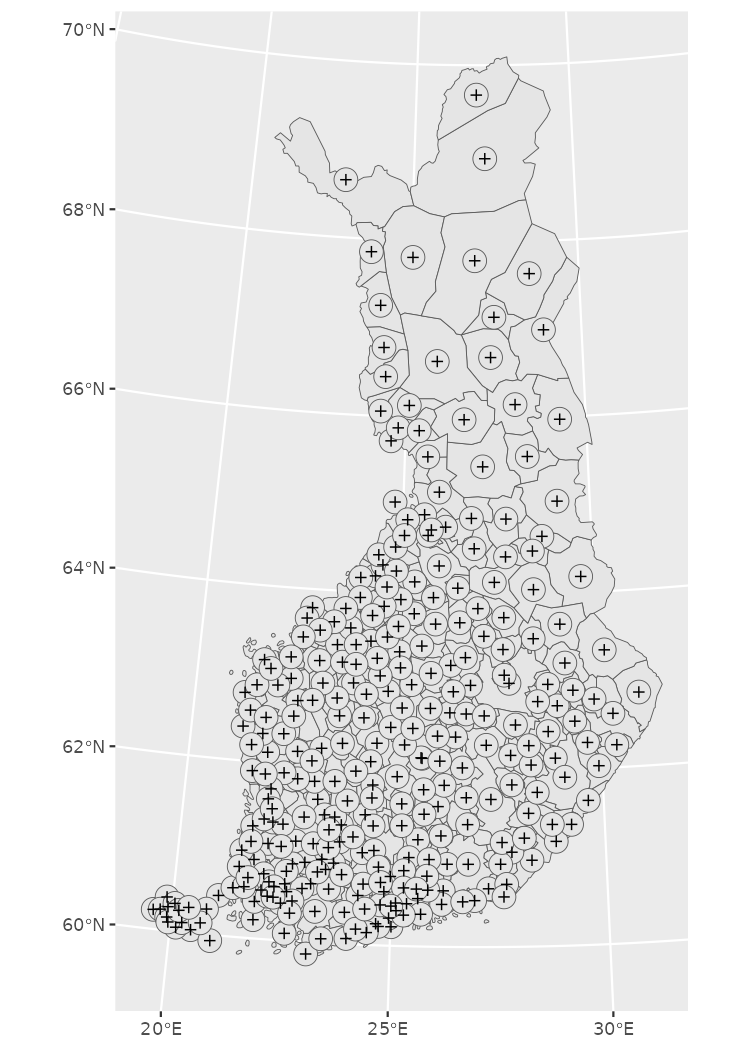

Creating regular grids

You can download predefined grids from Statistics Finland using get_statistical_grid and get_population_grid() -functions in geofi-package. These data contains not just the geographical shape, but also attribute data on population etc. within the grid cells.

However, you may need to create your own custom grid, for instance to aggregate your own point data, which can be created with st_make_grid() function.

As describes by Marko Kallio in Spatial data analysis with R.

It creates a regular grid over bounding box of an ‘sf’ object. Can be given a certain cell size, or number of cells in x and y directions. ‘what’ tells the function what kind of regular grid is wanted (polygons, corners, centers). Fishnets of lines rather than polygons can be created simply by casting the polygons as “LINESTRING”s. The resulting polygon grid is an ‘sfc’ object, so it needs to be made ‘sf’ in order for us to add the ID-attribute.

For this example we pick northern Muonio municipality and create a custom 2km*4km grid on top of it. Afterward we could aggregate the number of reindeer for each grid cell if we would have the data.

muonio <- muni %>% filter(municipality_name_fi == "Muonio")

grid_sf <- st_make_grid(muonio, cellsize = c(2000,4000), what="polygons") %>%
    st_sf()

grid_clip <- st_intersection(grid_sf, muonio)
grid_clip$rank <- 1:nrow(grid_clip)

ggplot(grid_clip) +
  geom_sf(aes(fill = rank), color = alpha("white", 1/3), size = 3) +
  scale_fill_viridis_c() +
  theme_minimal()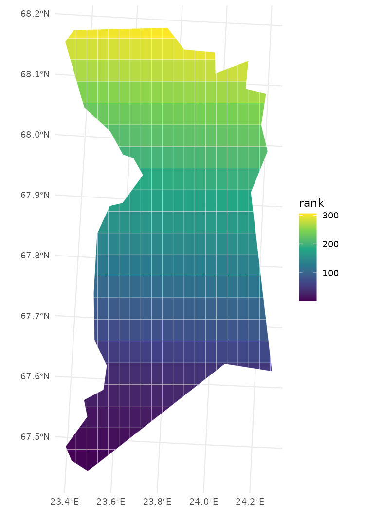

Voronoi polygons

In mathematics, a Voronoi diagram is a partition of a plane into regions close to each of a given set of objects. Source: Wikipedia: Voronoi diagram

Perhaps not the most useful operation, but worth taking a look as readily available in sf as function st_voronoi. In this case, it creates a layer of polygons that are closest to each municipality central locality.

library(geofi)
library(sf)

muni_voronoi <- municipality_central_localities %>% 
  st_union() %>%
  st_voronoi() %>% 
  st_cast() %>% 
  st_sf() %>% 
  st_intersection(st_union(muni)) %>% 
  mutate(rnk = 1:nrow(.))

ggplot(muni_voronoi) + 
  geom_sf(aes(fill = rnk)) +
  geom_sf(data = municipality_central_localities, shape = 4) +
  scale_fill_fermenter(palette = "YlGnBu") +
  theme_minimal() +
  theme(axis.text = element_blank(),
        axis.title = element_blank(),
        panel.grid = element_blank(),
        legend.position = "none")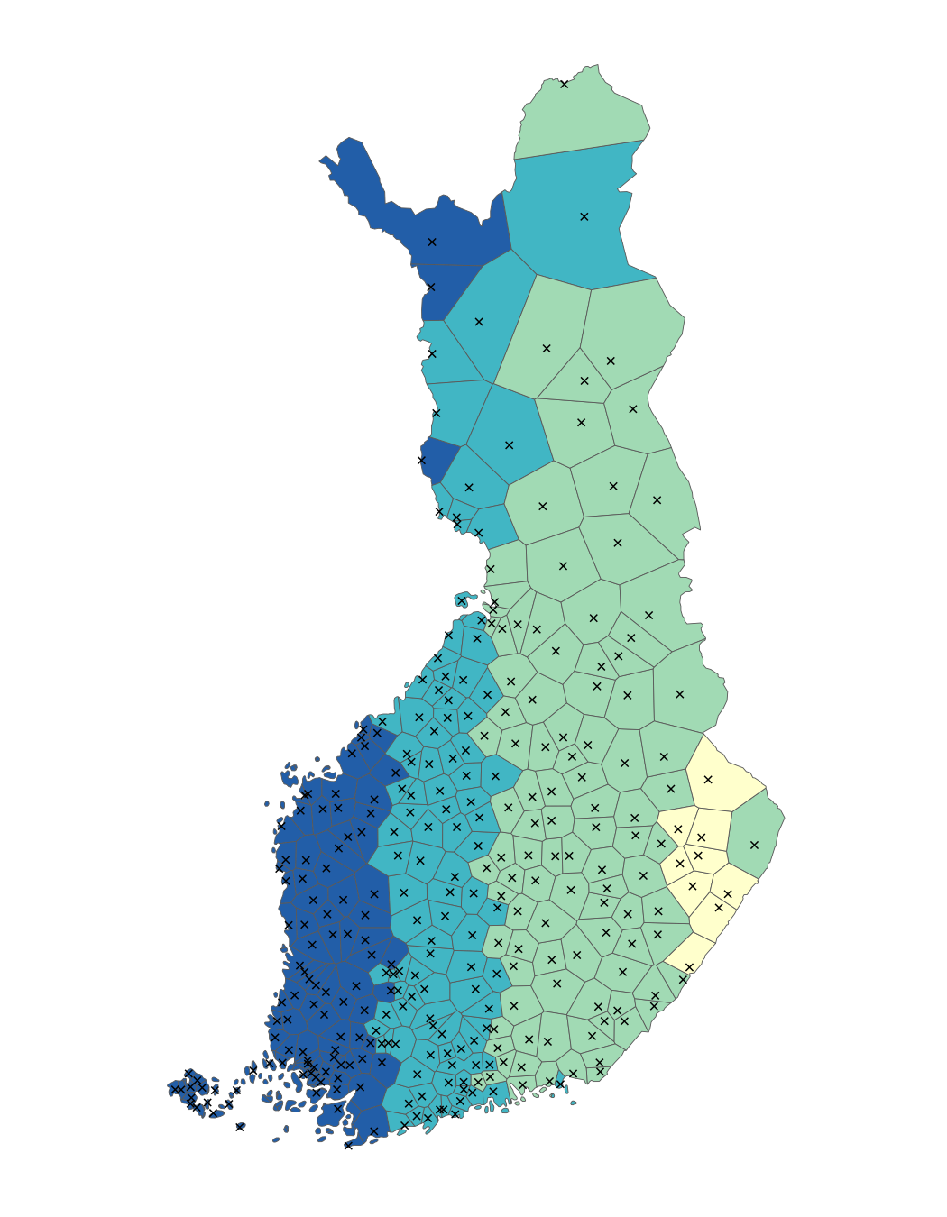

Calculating distances

Calculating distances is certainly at the core of geospatial analysis. In this exercise we are interested on calculating distances between municipality central localities in Finland. As expected, we are talking great circle distances here, ie. as the crow flies type of distances.

You can calculate distance matrices using st_distance()-function from sf-package that computes distances between pairs of geometries. geofi-package contains an internal data municipality_central_localities that we use to calculate distances between points.

First we need to subset the data and replace original municipality name column (teksti) with better from latest municipality key.

kunta <- geofi::municipality_central_localities %>%  
  select(teksti,kuntatunnus) %>%
  mutate(kuntatunnus = as.integer(kuntatunnus)) %>%
  select(-teksti) %>%
  left_join(geofi::municipality_key_2022 %>% select(municipality_code, municipality_name_fi),
            by = c("kuntatunnus" = "municipality_code")) %>%
  rename(teksti = municipality_name_fi)
kunta
#> Simple feature collection with 311 features and 2 fields
#> Geometry type: POINT
#> Dimension:     XY
#> Bounding box:  xmin: 91954.76 ymin: 6638646 xmax: 701036.8 ymax: 7755601
#> Projected CRS: ETRS89 / TM35FIN(E,N)
#> First 10 features:
#>    kuntatunnus    teksti                 geometry
#> 1          890   Utsjoki POINT (501086.5 7755601)
#> 2          498    Muonio   POINT (360886 7542117)
#> 3          148     Inari POINT (522136.3 7616266)
#> 4           47 Enontekiö POINT (362091.4 7589569)
#> 5          273    Kolari POINT (362088.2 7471921)
#> 6          976 Ylitornio POINT (350962.8 7359884)
#> 7          732     Salla POINT (573395.9 7413832)
#> 8          698 Rovaniemi   POINT (443256 7375804)
#> 9          854     Pello POINT (366564.7 7409490)
#> 10         320 Kemijärvi   POINT (519078 7399655)

Let’s aim at a data structure as below with both municipality name and code both from origin and destination.

origin_name	origin_code	destination_name	destination_code	dist_m
Helsinki	91	Espoo	92	15000
Vantaa	93	Espoo	92	18000
Espoo	92	Espoo	92	0

To get there lets create a for loop that calculates distance matrices from each municipality to all municipalities, assign each data to a list and finally bind the data frames into a single data.

d_list <- list()
kuntadatan_teksti_ja_kuntatunnus <- sf::st_drop_geometry(kunta) %>%
  select(teksti,kuntatunnus)
for (i in 1:nrow(kunta)){
  dist_tmp <- sf::st_distance(x = kunta[i,], y =  kunta)
  tibble(origin_name = kunta[i,]$teksti,
         origin_code = kunta[i,]$kuntatunnus) %>%
    bind_cols(kuntadatan_teksti_ja_kuntatunnus %>% rename(destination_name = teksti,
                                                          destination_code = kuntatunnus)) %>%
    mutate(dist = dist_tmp[1,]) -> d_list[[i]]
}
kunta_dist <- do.call("bind_rows", d_list) %>%
  mutate(dist = as.numeric(dist))
head(kunta_dist)
#> # A tibble: 6 × 5
#>   origin_name origin_code destination_name destination_code    dist
#>   <chr>             <int> <chr>                       <int>   <dbl>
#> 1 Utsjoki             890 Utsjoki                       890      0 
#> 2 Utsjoki             890 Muonio                        498 255404.
#> 3 Utsjoki             890 Inari                         148 140915.
#> 4 Utsjoki             890 Enontekiö                      47 216532.
#> 5 Utsjoki             890 Kolari                        273 315903.
#> 6 Utsjoki             890 Ylitornio                     976 423236.

Finally we can draw two plots to verify our results. First let’s draw a bar plot of 20 municipality central localities nearest to Helsinki

ggplot(kunta_dist %>%
         filter(origin_name == "Helsinki") %>%
         arrange(dist) %>% slice(1:20),
       aes(x = dist, y = reorder(destination_name, dist), label = round(dist))) +
         geom_col() + geom_text(aes(x = 1000), color = "white", hjust = 0) +
  labs(title = "Nearest 20 municipality localities to Helsinki", x = "distance in meters")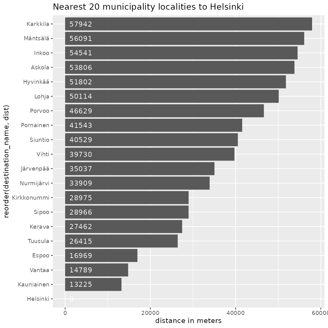

Then, lets find the municipality central locality that is nearest to the center of Finland.

# We firt need the country map as a single polygon
geofi::get_municipalities() %>% 
  sf::st_union() %>% 
  # then we need to compute the centroid of that polygon
  sf::st_centroid() -> fin_centroid

# The let's find the nearest neighbour with
distance <- st_distance(x = fin_centroid, y = kunta)
kuntadatan_teksti_ja_kuntatunnus %>% 
  mutate(dist = as.numeric(distance)) %>% 
  arrange(dist) -> closest_to_center
head(closest_to_center)
#>       teksti kuntatunnus     dist
#> 1 Siikalatva         791 13582.66
#> 2    Pyhäntä         630 17512.41
#> 3  Kärsämäki         317 33270.89
#> 4  Haapavesi          71 38730.91
#> 5      Vaala         785 50150.05
#> 6   Utajärvi         889 61041.41

And finally lets draw a bar plot of 20 furthest localities

furthest20 <- kunta_dist %>%
         filter(origin_name == closest_to_center[1,]$teksti) %>%
         arrange(desc(dist)) %>% slice(1:20)
ggplot(furthest20,
       aes(x = dist, y = reorder(destination_name, dist), label = round(dist))) +
  geom_col() + geom_text(aes(x = 10000), color = "white", hjust = 0) +
  labs(title = paste("Furthest 20 municipality localities \nfrom the most central locality of ", closest_to_center[1,]$teksti), x = "distance in meters")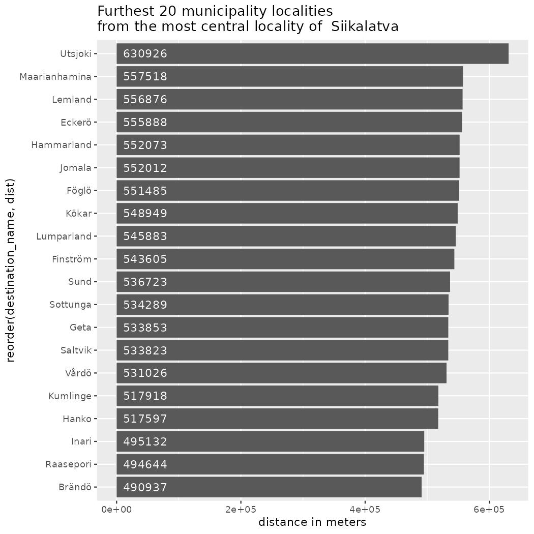

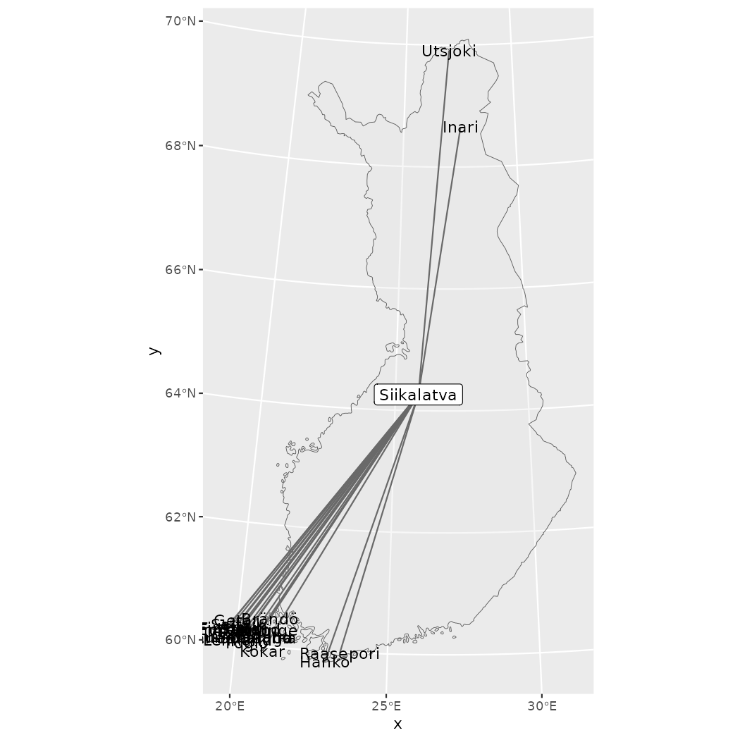
And at very last, we need to show those distances also on a map.

sf_lahto <- kunta %>% 
  filter(teksti %in% closest_to_center[1,]$teksti) %>%
  select(teksti)
sf_paate <- kunta %>% 
  filter(teksti %in% furthest20$destination_name) %>% 
  select(teksti)

triplst <- list()
for (i in 1:nrow(sf_paate)){
triplst[[i]] <- rbind(
  sf_lahto,
  sf_paate[i,]
) %>% 
  summarize(m = mean(row_number()),do_union=FALSE) %>% 
  st_cast("LINESTRING")
}
trips <- do.call("rbind", triplst)

ggplot() +
  geom_sf(data = muni %>% st_union(), alpha = .3) +
  geom_sf(data = trips, color = "dim grey") +
  geom_sf_label(data = sf_lahto, aes(label = teksti)) +
  geom_sf_text(data = sf_paate, aes(label = teksti))

Markus Kainu

2024-08-16